Introduction
Understanding if a device visited a place, brand, or type of store can be valuable context to have for your business. Companies we currently work with use store visit information to build custom audiences for advertising purposes, to better attribute ad campaign spend, and to send contextual push-notifications in real-time.
Unfortunately, accurately determining if a device visited a place can be a tough engineering problem to solve. Dealing with messy GPS data, incomplete business listing information, and limitations in knowing where places exactly are located make visit attribution a complex problem. However, building a visit attribution solution remains a worthwhile endeavor since it enables you to enrich digital data with physical-world context. Furthermore, building a visit attribution solution in-house allows you to tune the algorithm to your specific input data and specific use case which results in a better end solution for your customers.
Luckily, with SafeGraph Places, it’s become easier than ever to build your own robust visit attribution algorithm in-house.
In this white paper, learn about initial approaches taken to do visit attribution as well as potential drawbacks of these approaches. Then, learn about our current state-of- the-art visit attribution algorithm powered by SafeGraph Places.
Initial Approaches and Their Drawbacks
Let’s briefly cover a few simpler approaches and their potential drawbacks before presenting our current production solution.
Closest centroid wins
When SafeGraph first started working on visit attribution, it was very difficult to come across any building footprint (polygon) data, so we relied on points of interest (POI) centroid data. The algorithm we started with is as follows: for a given GPS ping, find the closest POI centroid and call it a visit to that POI if the distance is below some threshold.
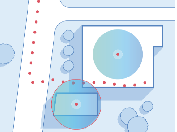
We have very consistently found that this “closest centroid wins” approach is only remotely comparable to other algorithms when you have large standalone stores (i.e. a Walmart surrounded by a large parking lot).
For a clear case where centroids aren’t good enough, think about an airport or a golf course, which don’t have an obvious centroid that you would want to use. There’s likely going to be another nearby location that’s closer, especially if you are near the edges of the large POI.Another good example is if you have large stores next to small stores as shown below. The centroids of the small stores will end up being closer just by virtue of having smaller footprints, which can bias your data.
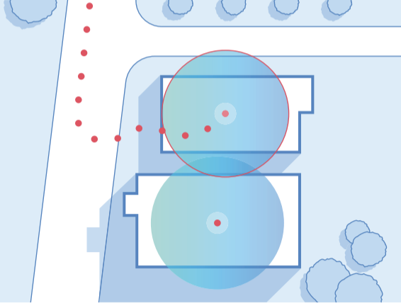
This is why any approach to accurately determining visits needs to take into account the actual building footprint (polygon), and not rely solely on a building’s centroid.This conclusion is the reason why SafeGraph decided to build out SafeGraph Places with building footprints for millions of global POIs.
Any ping inside a polygon is a visit
SafeGraph then tried the most simple polygon approach: a visit is just a sequence of GPS pings that are all inside of one POI polygon.
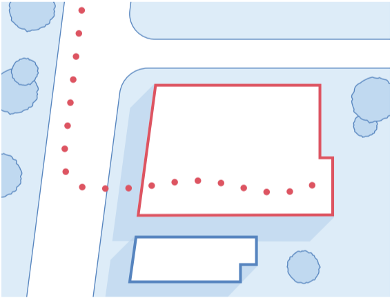
The biggest issue with this approach is that for most common POI, drifting GPS signals cause you to miss a lot of visits because the GPS pings will not always actually enter the building polygon. Even worse, they can drift into a neighboring building which will hurt your precision.
Another very common problem when we took this approach was devices that would switch back and forth between two locations, creating dozens of correct and incorrect visits that we would have to clean up after the fact.
One upside to this approach is that it works well for large places or outdoor places (airports, theme parks, etc) because any drift/noise in the GPS data is meaningless if the POI is big.
Any ping inside a custom geofence is a visit
Another common simple approach is to build custom geofences with padding around the POI that you care about, and then record any sequence of pings in that geofence as a visit.
By adding padding around the building polygon in your custom geofence, you can address some of the GPS drift issues. However, you still have a lot of potential precision issues. A device stopped at a red light next to one of your geofenced locations will show up as visiting that location, for example.
While you can add some filters to address the potential false positive visits, the new harder issue that you have to deal with is ambiguous matches. If you have two stores next to each other, either their geofences will overlap or the horizontal accuracy will make it so a device could have been in either place (or worse, both, one after the other).
The good news is you can use attributes such as:
- Time of day
- Duration spent in the geofence
- Distance from the pings to the building polygon
- Distance from the pings to the centroid
- Characteristics of the place (category, open hours, etc)
to try to predict which POI was the most likely visited (if any). This task is set up well for machine learning.
You can use features like the time of day interacting with the category of place (coffee shops are popular during different points in the day than bars are, for example), whether the location is open, if the duration was too short to be a visit, into account.
Overview of SafeGraph’s Visit Attribution Approach
Ultimately, SafeGraph’s solution involves segmenting the task of visits attribution into two distinct subproblems, both of which we feel closely model the processes a human might engage in if asked to create visits from GPS data.
At a high level, the solution can be decomposed as follows:
- Clustering GPS points such that every point in one cluster is associated with a visit to a single place
- Learning a model which can choose between a set of viable places
As we discuss below, our clustering processes take advantage of a modified version of the canonical DBSCAN clustering algorithm, re-tooled to more effectively deal with geospatial data that has a time component.
After clustering our GPS data and spatially joining it against our polygons, we’re left with the task of choosing the most-likely visit among a set of potential options. We found that this problem can be appropriately modeled by preference learning, and we developed a learning-to-rank model, similar to the technology used to power technologies like Google Search, that accurately learns how to rank a set of nearby places by comparing the feature vectors for those places.
Step #1: Cleaning GPS Data
Before we can even think about doing visits, we need to do some general data cleanup.
With GPS data, there are three primary prevalent issues:
- GPS signal drift
- Spiking horizontal accuracies
- “Jumpy” GPS pings (a ping going from point A to B faster than is possible)
The first one we will address as part of our algorithms below, but the next two are easier to address during a dedicated pre-processing step.
Spiking horizontal accuracies can happen for a lot of reasons. If a device loses GPS signal, it can either fall back to WiFi or the nearest cell tower. If WiFi is unavailable, it’s not uncommon for the horizontal accuracy to spike up above 1000m. This can be really problematic since a legitimate visit can be split into multiple components, or we can create incorrect visits in this new area. We spent some amount of time trying to make use of these high horizontal accuracy pings, but ultimately realized that the most accurate strategy is to just filter all horizontal accuracies above a tuned threshold.
There are a lot of reasons for jumpy GPS pings. The simplest explanation is that the data is fraudulent. Another possible explanation is that most phones will approximate your location based on the wifi information around you. If someone has recently moved, and a router that was previously in a different location is now near you, your phone may think it is wherever the last location of the router was, instead of where you are. In bad cases, this can look like a device moving from state to state rapidly.
Regardless of the reason for jumpy GPS pings, the approach is still the same. For any two points that are close in time, we compute a speed between them and if the speed is too high, we filter out the pings.
Finally, there’s one more filter we apply to the data before we can start clustering. We now will try to remove any non-stationary data. Since our goal is to create visits, we should be able to throw away any driving data.
To detect driving points, we combined two approaches:
1. You are looking for a sequence of points that are somewhat linear. To compute the linearity of a series of points (P₀, P₁, P₂, … Pn), we first compute the sum of sequential distances between all Pi and Pi+1: ∑ni=0d(Pi, Pi+1). We then divide this sum by the net distance traveled in the series: d(P0, PN). A value close to 1 indicates that the sequence is linear.
2. You can also calculate the speed between any two points pretty easily and filter for ones that are “too fast”. The reason you can’t just use this approach is you need to choose your threshold carefully so that noise or a few higher HA points don’t make it seem like the pings are driving when they aren’t.
Combining these, we essentially remove any sequence of pings that are too linear over a long enough period of time, and those that appear to be traveling too quickly.
Step #2: Clustering GPS Pings Together
The goal of this phase is to take all of our GPS data and try and turn it into potential visits, without using our places data. The key insight here is if you look at a series of GPS pings on a map with no places, you can generally figure out areas that a device could have visited.
You can also think of this as taking all your GPS pings and turning them into potential visits. By specifically solving just this component of the problem, the rest of the pipeline becomes a lot simpler because the ML model will only need to figure out which place is most likely as opposed to figuring out both which pings are relevant for a visit and then which location was the most likely. Also it severely reduces the data scale that you need to deal with.
For our approach, we started off with DBSCAN – a density based clustering algorithm which clusters points together based on how close they are.In DBSCAN, each ping is considered to either be part of a cluster or it is considered noise. The clusters that DBSCAN produces are essentially areas that the device was at for an extended period of time. You can control exactly what DBSCAN clusters mean by tuning the two hyper-parameters (one is the number of pings that need to be close together before it’s considered a cluster, and the other is the distance between two pings).
This works pretty well, but it’s missing one important element: time. If in the mornings you some location and then in the evenings you visit the location next door, we’d want those two to be part of different visits and therefore different clusters.
We took inspiration from a few papers written on the topic, and ultimately modified our DBSCAN algorithm to include time as follows:
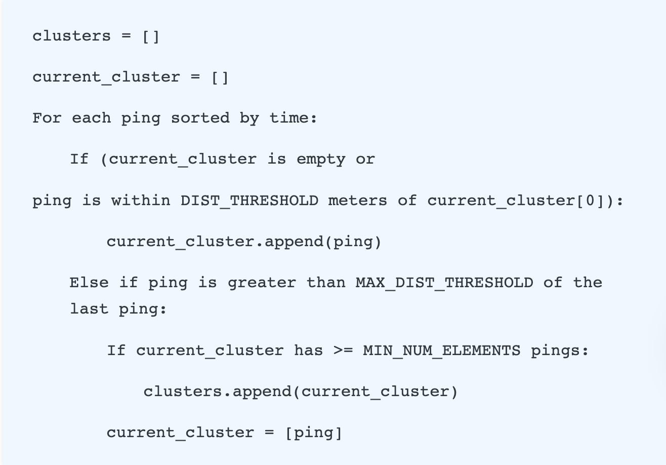
What this essentially says is that a sequence of pings that are within some DIST_THRESHOLD are considered a cluster as long as they never go more than MAX_DISTANCE_THRESHOLD away from the last ping and there are at least MIN_NUM_ELEMENTS in the cluster.
You should tune these parameters to best fit your data and use case. We found that DIST_THRESHOLD of 80m and MAX_DIST_THRESHOLD of 100m worked well for us.*
Refer back to step #1 on data cleanup for more information on making sure your data is clean enough to be put through the clustering process.
*Note this white paper was originally published with values of DIST_THRESHOLD = 100m and MAX_DIST_THRESHOLD = 300m, but these have been updated over time to A and B as the algorithm has undergone further refinement.
This approach generally works really well to cluster pings that are close together in both space and time. However, we found that there were two cases where we could do a little better:
1. The constraint that we have at least MIN_NUM_ELEMENTS in a cluster makes sense if you have no other information. However, if you have any additional information for any pings, you can turn those into their own clusters (or loosen the MIN_NUM_ELEMENTS constraint).
2. Large POI like airports pose a problem because their footprints are almost always going to be bigger than MAX_DIST_THRESHOLD so you pretty much always cut up your data.
The first problem is pretty straightforward to fix. For the second problem we ended up bringing back our “Any ping in a polygon is a visit” strategy, but just for POI with a really large area (which we found it to be really good at).
Bringing this altogether, what we ultimately do is:
1. General data clean from the previous step (remove high HA, jumpy pings, driving, etc)
2. Complete a first pass over the data, creating clusters out of consecutive pings that are in large POI
3. Do a second pass over the data, creating clusters from the remaining blocks of unused pings using our modified DBSCAN
4. Save the clusters, discard all unused pings
Step #3: Preparing the Clusters and their Possible Places
Now that we have clusters of potential visits, we need to add in our places information. We are trying to go from Dataset[Cluster] to Dataset[(Cluster, List[Places])] where the list of places is all the places that the cluster could have been referencing.
This step is relatively straightforward: we simply perform a geospatial join between our clusters and our polygons. You should make sure to add a buffer around the cluster to account for any horizontal accuracy uncertainty of the GPS pings.
Step #4: Predicting The Best Place For a Given Cluster
Motivation for framing problem as a ranking problem
After associating each cluster with a list of possible places, we’re left with the task of choosing between a set of viable options, some of which are more likely than others. This choice depends on a multitude of entangled features (such as the distance between cluster and polygon), lending itself well to machine learning.
The goal is to develop a machine learning system which takes as input (1) a cluster and (2) a list of places and which outputs the place associated with the cluster.
You might notice, though, that the problem structure laid out above doesn’t seem to fit nicely into those structures traditionally offered by off-the-shelf classification or prediction models. In prediction models, we input into the model some set of features (for instance, a set of features describing a cluster and an individual place) and output a continuous target variable — but it’s not clear exactly what the target variable should be in this case.
In classification, we classify a set of features with a label from a set that we’ve already learned; in this case, it’s not obvious what exactly the classifier is supposed to classify — a single place, one at a time? A set of places all together?
The problem structure becomes clearer, though, when we imagine how a human might perform this task:
Imagine being given the diagram to the right, in which a cluster C is surrounded by three potential places — Target, Walmart, and Bob’s Bar.
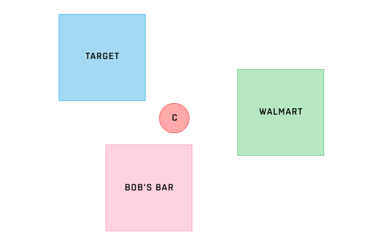
Visually, it seems unlikely that cluster C is a visit to Walmart. Importantly, we know this not merely because C is absolutely far from Walmart but because C is relatively far from Walmart, as compared to Target or Bob’s Bar.
This thought experiment indicates to us that choosing the correct visit is inherently a comparative exercise between places — that is, choosing a visit involves looking at the differences between sets of possible places. Thus, our feature set needs to somehow encapsulate these differences between places and not just raw place data itself.
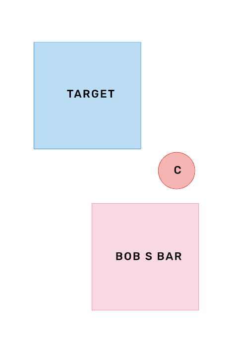
After ruling out Walmart, we’re left with the following situation:
Now we’re tasked with choosing between Target and Bob’s Bar.
This decision would likely be well informed by category and time-of-day information (for instance, we’re more likely to choose the bar if the cluster occurred at 11 p.m.), which we’ll return to shortly.
In the meantime, the takeaway here is that choosing the right place from an arbitrarily large set of options involves whittling down the option pool by comparing options between themselves. And this structure is one that can indeed be formalized in a way that’s more amenable to traditional ML techniques.
In fact, this problem is essentially isomorphic to any plain ol’ ranking problem, wherein your goal is to compute a ranking (also called an ordering) of an arbitrary large set of items. These models, of course, are ubiquitous, powering the rankings in technologies like Google Search, Yelp Restaurants, and Facebook’s People-You-May-Know.
Encoding ranking information
The key insight behind learning these models is to structure your feature set in such a way that it encodes ranking information. In the case of determining visits, we start by constructing a set of features for every pair. If a cluster matches against 8 possible places, this leaves us with 8 rows of features. Now we must manipulate this data to encode ordering information.
To encode ordering information between any two rows, A and B, we merely subtract B’s feature set from A’s. Training the model on these difference vectors helps it learn how to determine relative orderings between places. This is a standard technique in learning-to- rank called preference learning.
We set the label associated with this difference vector to be 1 if A was the true visit in our training data (thus, A should be ordered before B), -1 if B was the true visit in our training data (thus, B should be ordered before A), and 0 otherwise (that is, if neither A or B was the true visit in our training data). Ultimately, we filter out all 0 labels before training because we only care about finding the highest-ranked possible place and are not concerned with any orderings beyond that.
Our labels come from POI check-in data from a popular consumer app. By combining this check-in data with our GPS data, we’re able to construct clusters associated with each check-in. Because we know the true check-in, we’re aware which of the possible places was the true visit and which were non-visits. These “non-visits” form the negative examples in our training data.
Learning-to-rank model summary
To summarize what we’ve learned:
- For each cluster and possible place, create a set of features (that’s one row of features for each pair)
- Within this set, create all pairwise difference vectors — for N pairs, that’s (N * (N – 1)) / 2) difference vectors.
- For each pairwise difference vector A – B, set the label to 1 if A was the true visit, -1 if B was the true visit, and 0 otherwise.
- Filter out all 0 labels. This leaves us with (N – 1) rows with a 1 label and (N – 1) rows with a -1 label, giving us 2N – 2 rows in total.
- Learn a model on this set of features
As far as model choice is concerned, we borrowed inspiration from Microsoft Research and used a solution similar to the canonical LambdaMART architecture — that is, we built a gradient-boosted forest. We find these models to consistently strike the right tradeoff between being flexible enough to fit the data appropriately without learning noise, and all off-the-shelf learners have mechanisms in place (typically through hyper-parameters) to control regularization.
What’s more, we weren’t deterred by forests’ lack of interpretability because we were able to utilize libraries like ELI5 to pull out rich information about our model, such as feature importances.
Though we had an incredible amount of training data, we saw model performance plateau after ~50,000 training examples, which is small enough to feed into any standard tree library (though we used XGBoost).
Useful features for the model
We experimented with a large number of intuitive features and ultimately found the following set to be the most robust. Unsurprisingly, distance-related features had the most predictive validity.
DistanceToPlaceCentroid
- Distance between cluster centroid and place centroid
DistanceToPlaceWkt
- Distance between cluster centroid and nearest point on place WKT
- We include this feature in addition to DistanceToPlaceCentroid because there are cases (say, for relatively large polygons) in which the cluster is far from the centroid but close to the edge of the WKT, so failing to include this feature makes it seem as if the cluster is far away from the place when, in reality, it’s quite close
DistanceToPlaceCentroidRank
- Rank (e.g. 1st, 2nd, 3rd) of distance between cluster centroid and place centroid
- We chose to include rank-based features because we didn’t want our model to solely focus on the scale of the distance features
DistanceToPlaceWktRank
- Same as above, but for place WKT
NAICS x Hour
- Also, we created a large set of dummified features representing the interaction between the first 4 digits of each place’s NAICS code and the hour of day that the cluster occurred
- This intuition behind this set of features is you’re more likely to be seen at some types of places depending on the time. For instance, it’s likely that a cluster visited a nearby bar over a nearby Walmart if it’s 11 p.m. but more likely that a cluster visited the Walmart if it’s 11 a.m.
Using the output of the model to choose a visit
Because we’re creating pairwise combinations of feature vectors, we have more work to do after running our model over our features. We think of our model’s output as being similar to a round-robin tournament, in which every possible place “battles” every other possible place. Now we must combine the results from this round-robin tournament in such a way that we can choose a clear winner.
Our approach is simple: using the labels that our model predicted, we create essentially what amounts to a “tournament scorecard” — that is, a mapping between each possible place and the number of times it “won” when facing off against every other possible POI. The visit we choose is the merely the visit that has the most number of wins.
You may be wondering why we chose to perform ~N^2 comparisons instead of ~N. Similar to an algorithm that finds the maximum number in a list, our approach consisted of randomly choosing a possible place among those matched by a given cluster, calling it the “current champion,” and iteratively updating our understanding of the current champion by comparing it to other possible places. Unfortunately, though parsimonious, this approach isn’t valid because preference learning doesn’t guarantee transitivity. That is, our model may believe that place A should be ordered higher than place B, place B should be ordered higher than place C, and place C should be ordered higher than place A, thereby creating a cycle.
Because our model isn’t guaranteed to be transitive, performing ~N comparisons instead of ~N^2 isn’t robust. Thus, we recommend using a scorecard approach.
Below are the final set of steps we use in the production ML pipeline to choose a visit:
- For each cluster, create a row of features for each possible place using the feature set outlined above
- Create all pairwise difference vectors between this set of raw features
- Run each difference vector through the model, which will output 1 if it thinks that the left-hand feature vector should be ordered higher than the right-hand vector and -1 if the right-hand should be ordered before the left-hand.
- Using these labels, create a scorecard that associated each possible place with the number of times it “won” a face-off
- Choose the final visit to be the one that won the most number of times
Benchmarking performance
Ultimately, we care about our ability to choose the correct visit among a set of potential options, so we benchmarked our performance on this task relative to a set of classifiers that are less sophisticated.
In particular, we compared ourselves to classifiers that
1. Chose a visit at random from the pool of viable options and
2. Chose the polygon that was closest to the cluster center.
Of course, performance for these strategies varies largely as a function of the number of possible places that were matched to each cluster in the first place (in other words, choosing the correct visit among a set of 2 options is significantly easier than for a set of 10).
From benchmarking, we found our model significantly outperforms both naive classifiers, though the distance-based classifier performs admirably as well.